Case Study: AVL Trees

AVL Trees

An AVL tree is defined by the following Haskell datatype:¹

While the Haskell type signature describes any old binary tree, an AVL tree like that shown in Figure 1.1 actually satisfies two crucial invariants: it should be binary search ordered and balanced.

Figure 1.1: An AVL tree is an ordered, height-balanced tree.

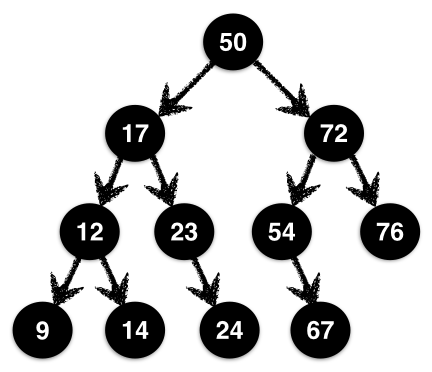
A Binary Search Ordered tree is one where at each Node, the values of the left and right subtrees are strictly less and greater than the values at the Node. In the tree in Figure 1.1 the root has value 50 while its left and right subtrees have values in the range 9-23 and 54-76 respectively. This holds at all nodes, not just the root. For example, the node 12 has left and right children strictly less and greater than 12.

A Balanced tree is one where at each node, the heights of the left and right subtrees differ by at most 1. In Figure 1.1, at the root, the heights of the left and right subtrees are the same, but at the node 72 the left subtree has height 2 which is one more then the right subtree.

Order ensures that there is at most a single path of left and right moves from the root at which an element can be found; balance ensures that each such path in the tree is of size \(O(\log\ n)\) where \(n\) is the numbers of nodes. Thus, together they ensure that the collection operations are efficient: they take time logarithmic in the size of the collection.

Specifying AVL Trees

The tricky bit is to ensure order and balance. Before we can ensure anything, let’s tell LiquidHaskell what we mean by these terms, by defining legal or valid AVL trees.

To Specify Order we just define two aliases AVLL and AVLR – read AVL-left and AVL-right – for trees whose values are strictly less than and greater than some value X:

The Real Height of a tree is defined recursively as 0 for Leafs and one more than the larger of left and right subtrees for Nodes. Note that we cannot simply use the ah field because that’s just some arbitrary Int – there is nothing to prevent a buggy implementation from just filling that field with 0 everywhere. In short, we need the ground truth: a measure that computes the actual height of a tree. ²

A Reality Check predicate ensures that a value v is indeed the real height of a node with subtrees l and r:

A Node is $n$-Balanced if its left and right subtrees have a (real) height difference of at most \(n\). We can specify this requirement as a predicate isBal l r n

A Legal AVL Tree can now be defined via the following refined data type, which states that each Node is \(1\)-balanced, and that the saved height field is indeed the real height:

Smart Constructors

Lets use the type to construct a few small trees which will also be handy in a general collection API. First, let’s write an alias for trees of a given height:

An Empty collection is represented by a Leaf, which has height 0:

As you can imagine, it can be quite tedious to keep the saved height field ah in sync with the real height. In general in such situations, which arose also with lazy queues, the right move is to eschew the data constructor and instead use a smart constructor that will fill in the appropriate values correctly. ³

The Smart Constructor node takes as input the node’s value x, left and right subtrees l and r and returns a tree by filling in the right value for the height field.

Hint: Think about the (refined) type of the actual constructor Node, and the properties it requires and ensures.

Inserting Elements

Next, let’s turn our attention to the problem of adding elements to an AVL tree. The basic strategy is this:

1. Find the appropriate location (per ordering) to add the value,
2. Replace the Leaf at that location with the singleton value.

If you prefer the spare precision of code to the informality of English, here is a first stab at implementing insertion: ⁴

Unfortunately insert0 does not work. If you did the exercise above, you can replace it with mkNode and you will see that the above function is rejected by LiquidHaskell. The error message would essentially say that at the calls to the smart constructor, the arguments violate the balance requirement.

Insertion Increases The Height of a sub-tree, making it too large relative to its sibling. For example, consider the tree t0 defined as:

ghci> let t0 = Node { key = 'a'
                    , l   = Leaf
                    , r   = Node {key = 'd'
                                 , l  = Leaf
                                 , r  = Leaf
                                 , ah = 1 }
                    , ah = 2}

If we use insert0 to add the key 'e' (which goes after 'd') then we end up with the result:

ghci> insert0 'e' t0
  Node { key = 'a'
       , l   = Leaf
       , r   = Node { key = 'd'
                    , l   = Leaf
                    , r   = Node { key = 'e'
                                 , l   = Leaf
                                 , r   = Leaf
                                 , ah  = 1   }
                    , ah = 2                 }
       , ah = 3}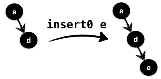

Figure 1.2: Naive insertion breaks balancedness

In the above, illustrated in Figure 1.2 the value 'e' is inserted into the valid tree t0; it is inserted using insR0, into the right subtree of t0 which already has height 1 and causes its height to go up to 2 which is too large relative to the empty left subtree of height 0.

LiquidHaskell catches the imbalance by rejecting insert0. The new value y is inserted into the right subtree r, which (may already be bigger than the left by a factor of 1). As insert can return a tree with arbitrary height, possibly much larger than l and hence, LiquidHaskell rejects the call to the constructor node as the balance requirement does not hold.

Two lessons can be drawn from the above exercise. First, insert may increase the height of a tree by at most 1. So, second, we need a way to rebalance sibling trees where one has height 2 more than the other.

Rebalancing Trees

The brilliant insight of Adelson-Velsky and Landis was that we can, in fact, perform such a rebalancing with a clever bit of gardening. Suppose we have inserted a value into the left subtree l to obtain a new tree l' (the right case is symmetric.)

The relative heights of l' and r fall under one of three cases:

• (RightBig) r is two more than l',
• (LeftBig) l' is two more than r, and otherwise
• (NoBig) l' and r are within a factor of 1,

We can specify these cases as follows.

the function getHeight accesses the saved height field.

In insL, the RightBig case cannot arise as l' is at least as big as l, which was within a factor of 1 of r in the valid input tree t. In NoBig, we can safely link l' and r with the smart constructor as they satisfy the balance requirements. The LeftBig case is the tricky one: we need a way to shuffle elements from the left subtree over to the right side.

What is a LeftBig tree? Lets split into the possible cases for l', immediately ruling out the empty tree because its height is 0 which cannot be 2 larger than any other tree.

• (NoHeavy) the left and right subtrees of l' have the same height,
• (LeftHeavy) the left subtree of l' is bigger than the right,
• (RightHeavy) the right subtree of l' is bigger than the left.

The Balance Factor of a tree can be used to make the above cases precise. Note that while the getHeight function returns the saved height (for efficiency), thanks to the invariants, we know it is in fact equal to the realHeight of the given tree.

Heaviness can be encoded by testing the balance factor:

Adelson-Velsky and Landis observed that once you’ve drilled down into these three cases, the shuffling suggests itself.

Figure 1.3: Rotating when in the LeftBig, NoHeavy case.

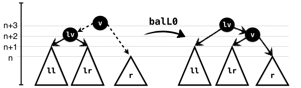
In the NoHeavy case, illustrated in Figure 1.3, the subtrees ll and lr have the same height which is one more than that of r. Hence, we can link up lr and r and link the result with l. Here’s how you would implement the rotation. Note how the preconditions capture the exact case we’re in: the left subtree is NoHeavy and the right subtree is smaller than the left by 2. Finally, the output type captures the exact height of the result, relative to the input subtrees.

Figure 1.4: Rotating when in the LeftBig, LeftHeavy case.

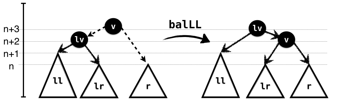
In the LeftHeavy case, illustrated in Figure 1.4, the subtree ll is larger than lr; hence lr has the same height as r, and again we can link up lr and r and link the result with l. As in the NoHeavy case, the input types capture the exact case, and the output the height of the resulting tree.

Figure 1.5: Rotating when in the LeftBig, RightHeavy case.

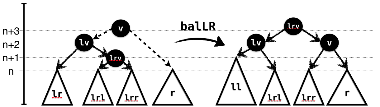
In the RightHeavy case, illustrated in Figure 1.5, the subtree lr is larger than ll. We cannot directly link it with r as the result would again be too large. Hence, we split it further into its own subtrees lrl and lrr and link the latter with r. Again, the types capture the requirements and guarantees of the rotation.

The RightBig cases are symmetric to the above cases where the left subtree is the larger one.

To Correctly Insert an element, we recursively add it to the left or right subtree as appropriate and then determine which of the above cases hold in order to call the corresponding rebalance function which restores the invariants.

The refinement, eqOrUp says that the height of t is the same as s or goes up by at most 1.

The hard work happens inside insL and insR. Here’s the first; it simply inserts into the left subtree to get l' and then determines which rotation to apply.

Refactoring Rebalance

Next, let’s write a function to delete an element from a tree. In general, we can apply the same strategy as insert:

1. remove the element without worrying about heights,
2. observe that deleting can decrease the height by at most 1,
3. perform a rotation to fix the imbalance caused by the decrease.

We painted ourselves into a corner with insert: the code for actually inserting an element is intermingled with the code for determining and performing the rotation. That is, see how the code that determines which rotation to apply – leftBig, leftHeavy, etc. – is inside the insL which does the insertion as well. This is correct, but it means we would have to repeat the case analysis when deleting a value, which is unfortunate.

Instead let's refactor the rebalancing code into a separate function, that can be used by both insert and delete. It looks like this:

The bal function is a combination of the case-splits and rotation calls made by insL (and ahem, insR); it takes as input a value x and valid left and right subtrees for x whose heights are off by at most 2 because as we will have created them by inserting or deleting a value from a sibling whose height was at most 1 away. The bal function returns a valid AVL tree, whose height is constrained to satisfy the predicate reBal l r t, which says:

• (bigHt) The height of t is the same or one bigger than the larger of l and r, and
• (balHt) If l and r were already balanced (i.e. within 1) then the height of t is exactly equal to that of a tree built by directly linking l and r.

Insert can now be written very simply as the following function that recursively inserts into the appropriate subtree and then calls bal to fix any imbalance:

Deleting Elements

Now we can write the delete function in a manner similar to insert: the easy cases are the recursive ones; here we just delete from the subtree and summon bal to clean up. Notice that the height of the output t is at most 1 less than that of the input s.

The tricky case is when we actually find the element that is to be removed. Here, we call merge to link up the two subtrees l and r after hoisting the smallest element from the right tree r as the new root which replaces the deleted element x.

getMin recursively finds the smallest (i.e. leftmost) value in a tree, and returns the value and the remainder tree. The height of each remainder l' may be lower than l (by at most 1.) Hence, we use bal to restore the invariants when linking against the corresponding right subtree r.

Functional Correctness

We just saw how to implement some tricky data structure gymnastics. Fortunately, with LiquidHaskell as a safety net we can be sure to have gotten all the rotation cases right and to have preserved the invariants crucial for efficiency and correctness. However, there is nothing in the types above that captures “functional correctness”, which, in this case, means that the operations actually implement a collection or set API, for example, as described here. Lets use the techniques from that chapter to precisely specify and verify that our AVL operations indeed implement sets correctly, by:

1. Defining the set of elements in a tree,
2. Specifying the desired semantics of operations via types,
3. Verifying the implementation. ⁵

We’ve done this once before already, so this is a good exercise to solidify your understanding of that material.

The Elements of an AVL tree can be described via a measure defined as follows:

Let us use the above measure to specify and verify that our AVL library actually implements a Set or collection API.